Networks - Introduction

Download Chapter PDF

Download Chapter notebook (ipynb)

Mandatory Lesson Feedback Survey

Overview

Questions

• How are graphs represented?
• How are graphs visualised?
• What are common types of graphs?

Objectives

• Understanding the notion of a graph
• Explaining nodes and edges represent networks
• The network matrix formalism
• Visualising graphs
• Understanding undirected, directed and bipartite graphs

Prerequisites

• Basic Python
• Basic Matplotlib

Example: Protein-protein interactions

---

Protein-protein interactions (PPIs) (PLoS: Protein–Protein Interactions) refer to specific functional or physical contact between proteins in vivo. Interactions may be dependent on biological context, organism, definition of interaction, and many other factors. An example of PPIs can be seen below.

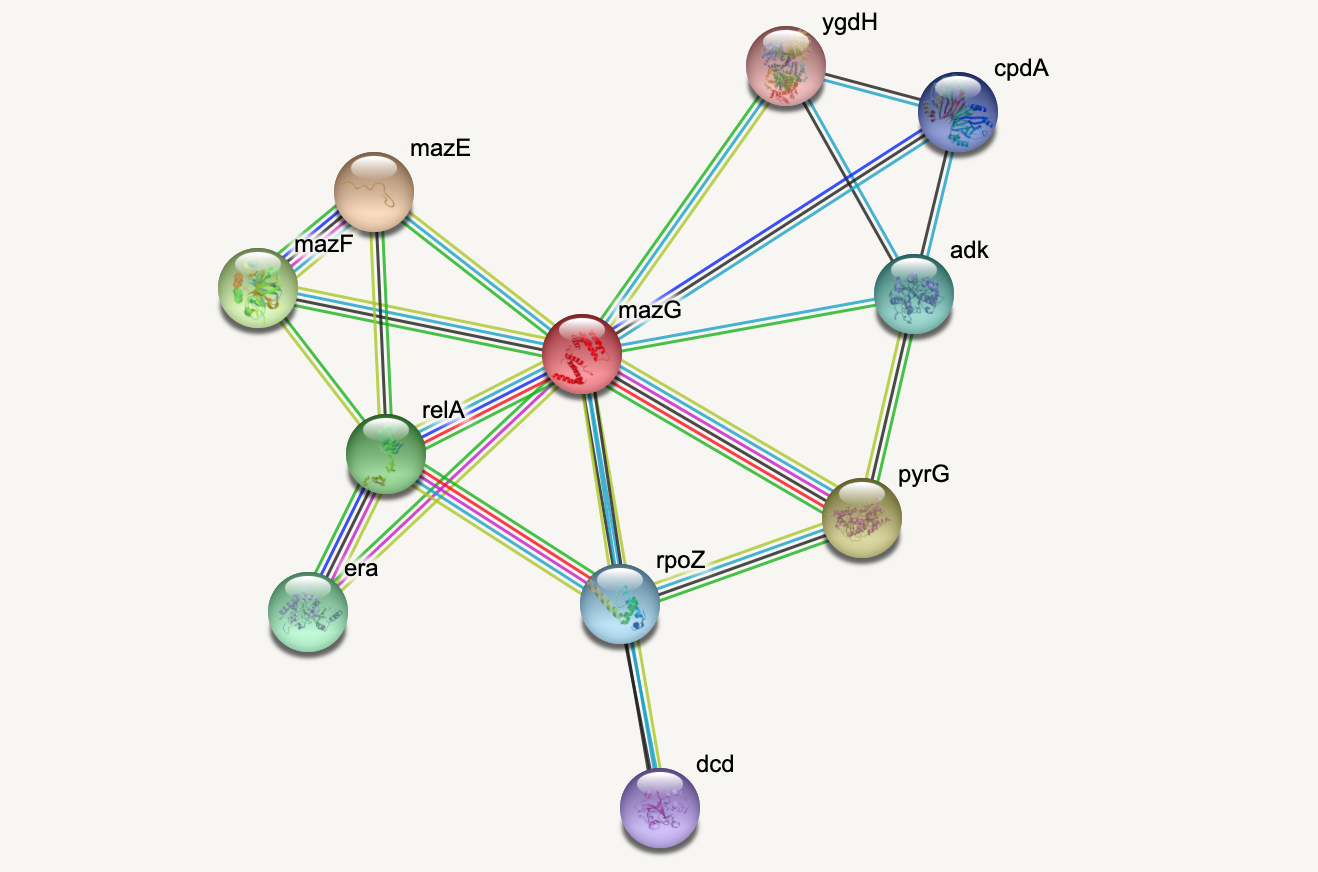
PPIs may be conceptualised as a network, in order to give greater context to the protein interactions, and to see how changes to one protein may affect another protein several steps removed. A PPI network can be modelled via a graph in which the nodes represent the proteins and the edges represent interactions: an edge from node A to node B indicates protein B interacts with protein A. The diagram above shows the PPI network centred around the protein \(mazG\) in Escherichia coli K12 MG1655. This is part of a toxin-antitoxin system. These systems generally encode pairs of toxin and inhibitory antitoxin proteins, are transmitted by plasmids, and likely serve several biological functions including stress tolerance and genome stabilisation. \(mazG\) regulates the type II toxin-antitoxin system shown in this network, where \(mazF\) is the toxin and \(mazE\) is the antitoxin. More details on the proteins in this network can be seen on STRING-DB (STRING-DB: mazG in E. coli.

At the end of this lesson we are going to use Python to draw this PPI network. Before this however, we shall begin with some examples to familiarise you with the elements and properties of graphs.

An Introduction to Networks

---

What is a graph?

A graph is an object in mathematics to describe relationships between objects. A simple example of a visual representation of a graph is given below.

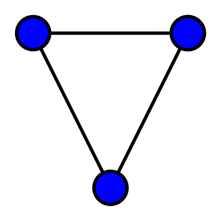
This graph contains three objects - nodes or vertices - and three links - edges or arcs - between the nodes. Graphs can be used to represent networks. For a formal definition of a graph see, e.g. the Wikipedia entry.

If the above graph represented a protein-protein interaction network then the nodes would represent three proteins and the edges represent interactions between them. To add further proteins, you add new nodes to the network. To include further dependencies (when there are more nodes), you add edges.

We shall see below how we can build, modify and represent networks in Python.

NetworkX

NetworkX is a Python package for the creation, manipulation, and study of the structure, dynamics, and functions of complex networks.

To use NetworkX and visualise your networks, you can import the whole package.

PYTHON

import networkx as nx
from matplotlib.pyplot import show

Nodes and Edges

Nodes are a basic unit of network data, and are linked to other nodes by edges, which show the way(s) in which the nodes are connected or related. In NetworkX, a range of Python objects, including numbers, text strings, and networks can be nodes.

Let’s start by creating an empty graph object and then add some nodes to it.

PYTHON

firstGraph = nx.Graph()

firstGraph.add_node('Node A')
firstGraph.add_node('Node B')
firstGraph.add_node('Node C')

print(type(firstGraph))
print('')
print(firstGraph.nodes)
print('')

OUTPUT

<class 'networkx.classes.graph.Graph'>

['Node A', 'Node B', 'Node C']

We have created a graph called firstGraph, added three nodes, and then printed the type of object and a list of the nodes in this graph. So far, these nodes have no relationship to each other? To specify relationships (representing e.g. interactions) we can add edges to show how the nodes are connected.

PYTHON

firstGraph.add_edge('Node A', 'Node B')
firstGraph.add_edge('Node A', 'Node C')
firstGraph.add_edge('Node B', 'Node C')

print(firstGraph.edges)

OUTPUT

[('Node A', 'Node B'), ('Node A', 'Node C'), ('Node B', 'Node C')]

Here we created edges between Nodes A and B, A and C, and B and C, and printed a list of these edges. We can also get a summary of how many nodes and edges our graph currently has. At this stage, our graph should have three nodes and three edges. Here is how to check that in NetworkX.

PYTHON

firstGraph.number_of_nodes()

OUTPUT

3

PYTHON

firstGraph.number_of_edges()

OUTPUT

3

Visualising networks

We have a basic graph called firstGraph, so let’s visualise it. In NetworkX, we can use function draw.

PYTHON

nx.draw(firstGraph)
show()

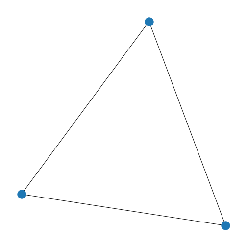
With the default settings, we get a triangle with three blue nodes in the corners, connected by three lines. There are no arrowheads on the lines, the network is therefore referred to as undirected.

To make the graph less abstract, we can add labels to the nodes. This is done setting up a dictionary where we use as keys the names given to the nodes when they were set up. The single value is the label to be used for the display.

Through NetworkX we can also dictate the way the nodes are positioned by setting a layout. There are many options, and we are using the spiral layout as an example. For a list of layout options, please check the NetworkX documentation.

PYTHON

firstGraphLayout = nx.spiral_layout(firstGraph)

firstGraphLabels = {
#   key     : value
    'Node A': 'A',
    'Node B': 'B',
    'Node C': 'C',
}

nx.draw(firstGraph, firstGraphLayout,
        labels=firstGraphLabels)

show()

Note

We use draw providing the graph object followed by the (optional) layout as positional arguments. Other keyword arguments (here the labels) are then added, separated by comma.

Saving Figures

If you want to save a network graph to a file, you can use function savefig. Here is an example that will save the figure in the folder with the code.

PYTHON

from matplotlib.pyplot import savefig

PYTHON

firstGraphLayout = nx.spiral_layout(firstGraph)

firstGraphLabels = {
    'Node A': 'A',
    'Node B': 'B',
    'Node C': 'C',
}

nx.draw(firstGraph, firstGraphLayout,
        labels=firstGraphLabels)

savefig('my_network.png', format='png');

show()

You may want to alter the appearance of your graph in different ways. Let’s say you want the nodes to be red: you achieve this by using the keyword argument node_color.

PYTHON

nx.draw(firstGraph, firstGraphLayout,
        labels=firstGraphLabels,
        node_color='r')

show()

Note that, as always, the spelling is the US version, ‘color’.

Creating a Network Matrix

---

A generic way to define graphs is via a two dimensional array known as the network matrix or adjacency matrix. We won’t go into the details of matrices here but will just show you how to create them in Python.

For our purpose a matrix is a collection of numbers. Let us start by creating a matrix that contains only zeroes. A very easy way to create a matrix with zeroes in Python is using zeros from Numpy. The number of network nodes is equal to the number of rows and columns in the array.

PYTHON

from numpy import zeros

nodes = 3

my_matrix = zeros((nodes, nodes))

print(my_matrix)

OUTPUT

[[0. 0. 0.]
 [0. 0. 0.]
 [0. 0. 0.]]

We have given the zeros function two arguments, 3 and 3, and it has created an array of 9 numbers (all of value 0) arranged into 3 rows and 3 columns. This is a square matrix because the number of rows is equal to the number of columns. We say that this matrix is of dimension \(3\times 3\).

To check the dimensions of a Numpy array, you can use shape. Since in the above code we have assigned the matrix to the variable my_matrix we can call it as follows.

PYTHON

my_matrix.shape

OUTPUT

(3, 3)

Note

Note that shape does not take arguments. It returns the dimensions of the matrix as an array of length 2; the first element is the number of rows and the second element is the number of columns.

We can now access each element of my_matrix and change its value. To change the element in the second row and the third column we use the syntax my_matrix[1, 2] where we first specify the row index and the column index second, separated by a comma.

PYTHON

my_matrix[2, 0] = 1
my_matrix[1, 0] = 1

print(my_matrix)

OUTPUT

[[0. 0. 0.]
 [1. 0. 0.]
 [1. 0. 0.]]

Do it Yourself

Create a 4x4 matrix called \(n\) and set the elements \(n_{0,1}=1\), \(n_{1,2}=1\) and \(n_{1,3}=1\).

DIY ANSWER

PYTHON

n = zeros((4,4))

n[0, 1] = 1
n[1, 2] = 1
n[1, 3] = 1

print(n)

OUTPUT

[[0. 1. 0. 0.]
 [0. 0. 1. 1.]
 [0. 0. 0. 0.]
 [0. 0. 0. 0.]]

Representing graphs

---

Now we shall see how a \(3 \times 3\) square matrix can represent a graph with three nodes which we call \(A\), \(B\) and \(C\). Consider the following table where we have taken the matrix elements and labelled both the rows and the columns \(A,B\) and \(C\).

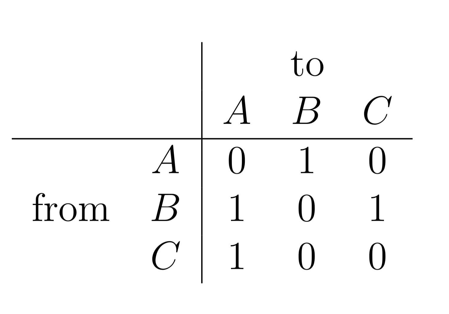
This matrix can represent a graph with three nodes. The value of 1 in the first row and the second column indicates that there is an edge from node \(A\) to node \(B\). Therefore, the row position indicates the node that an edge emanates from and the column position indicates the node that the edge ends on.

We can see that there are four edges in this graph:

• from node \(A\) to node \(B\)

• from node \(B\) to node \(A\)

• from node \(B\) to node \(C\)

• from node \(C\) to node \(A\)

Do it Yourself

For the matrix, \(n\), created in Exercise 1.1, is a network matrix representing a graph, use code to check the number of nodes and edges.

DIY ANSWER

The graph has four nodes and three edges.
$n_{0,1} $ or $n[0][1]$ is an edge from node 0 to node 1.
$n_{1,2}$ or $n[1][2]$ is an edge from node 1 to node 2.
$n_{1,3}$ or $n[1][3]$ is an edge from node 1 to node 3.

Different Layouts for Visualisation

---

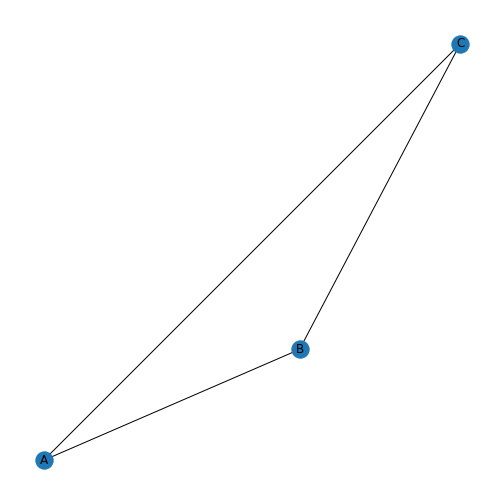
Now that we know how to create a matrix which can represent the graph, we want to know what the graph coming from this matrix looks like.

First, we set up the network (or: adjacency) matrix in the above table from scratch. Then we use NetworkX function from_numpy_matrix to turn our matrix into a NetworkX Graph object called new_graph. We set the layout to a spiral layout (as we did before) and then draw the graph.

PYTHON

new_matrix = zeros((3,3))

new_matrix[1, 2] = 1
new_matrix[2, 0] = 1
new_matrix[0, 1] = 1
new_matrix[1, 0] = 1

new_graph = nx.from_numpy_matrix(new_matrix)

newLayout = nx.spiral_layout(new_graph)

nx.draw(new_graph, newLayout)

show()

We haven’t specified labels. We can specify the labels using a dictionary. Let us first see how the nodes are stored to find their Python names.

PYTHON

list(new_graph.nodes)

OUTPUT

[0, 1, 2]

By default, the nodes are given the names of their indices. We can refer to these indices and assign labels.

PYTHON

newLabels = {
# key : value
    0: 'A',
    1: 'B',
    2: 'C',
}

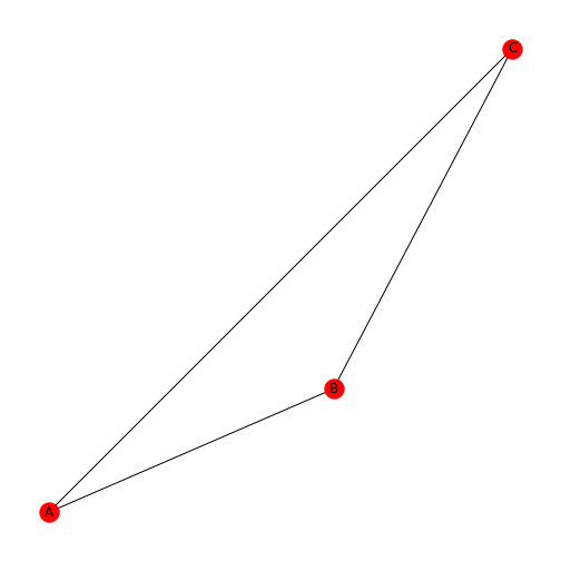
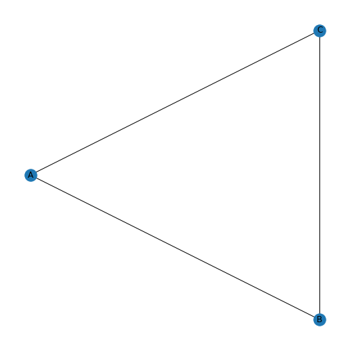
We can now draw the graph again, and specify the new labels A, B, and C.

PYTHON

nx.draw(new_graph, newLayout,
        labels=newLabels)

show()

There are many different options available for drawing graphs. Use help(nx.draw) to get a description of the options available for the graph as a whole, the nodes and the edges.

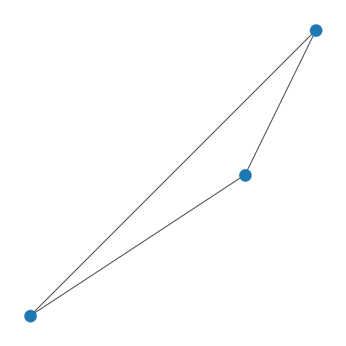
We shall first experiment with the graph layout. Converting a mathematical description of a graph, i.e. an adjacency matrix, to a graphical description is a difficult problem, especially for large graphs. The algorithms that perform this operation are known as graph layout algorithms and NetworkX has many of them implemented. We used spiral_layout to produce the drawing above. Further specifications can be made within each layout, and you can access the details with \(help\).

Some graph layout algorithms have a random component such as the initial position of the nodes. This means that different realisations of the layouts will not be identical.

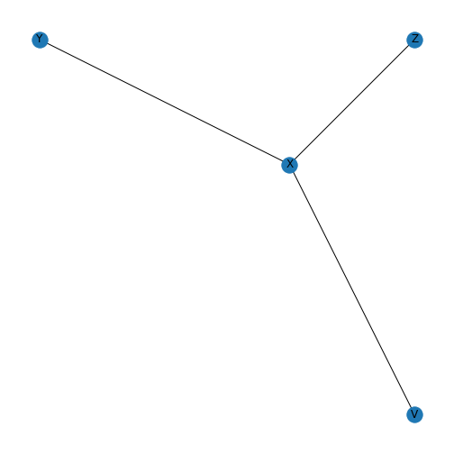
Do it Yourself

1. Use the graph layout algorithm called shell_layout to plot new_graph.

2. Draw the graph with a third layout algorithm called random_layout. Execute the code to draw the graph several times.

3. Draw the graph from the matrix \(n\), created in Exercise 1.1 with the layout algorithm spectral_layout. Give the nodes the names \(V\), \(X\), \(Y\) and \(Z\).

Q1

PYTHON

newLayout = nx.shell_layout(new_graph)

nx.draw(new_graph, newLayout,
        labels=newLabels)

show()

Q2

PYTHON

newLayout = nx.random_layout(new_graph)

nx.draw(new_graph, newLayout)

show()

PYTHON

# The layout of this graph changes each time you run the code.

Q3

PYTHON

n = zeros((4,4))

n[0, 1] = 1
n[1, 2] = 1
n[1, 3] = 1

new = nx.from_numpy_matrix(n)

newLabels = {
    0: 'V',
    1: 'X',
    2: 'Y',
    3: 'Z',
}

newLayout = nx.spectral_layout(new)

nx.draw(new, newLayout,
        labels=newLabels)

show()

Customising nodes and edges

---

Now we are going to look at some ways to access and change some properties, or attributes, of the nodes in the graph. We have already changed the node colour from blue to red. Let’s say we want to change the colour to gold (for a list of available names see matplotlib: plot colours), change the node shapes to hexagons (matplotlib: node shapes), and increase the node size. This plot will vary each time you run it, due to the layout algorithm.

PYTHON

new_graph = nx.from_numpy_matrix(new_matrix)

newLayout = nx.random_layout(new_graph)

newLabels = {
    0: 'A',
    1: 'B',
    2: 'C',
}

nx.draw(new_graph, newLayout,
        labels=newLabels,
        node_color='gold',
        node_shape="H",
        node_size=2000)
show()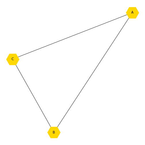

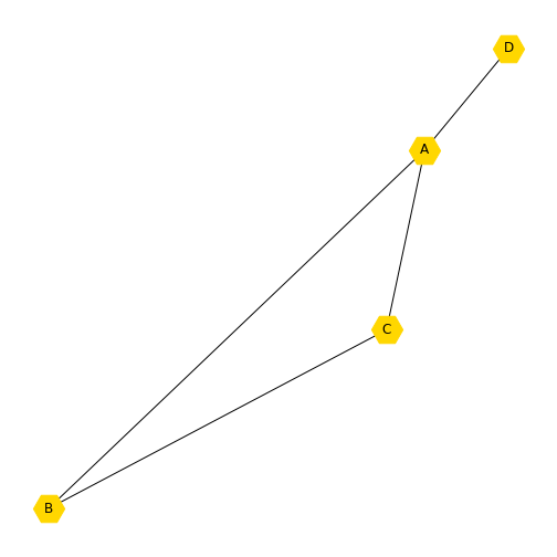
You may want to add another node, but only have it connected to one of the existing nodes. Here we add a new node, which is the number 3 (because Python indexes from zero). You can print the nodes and see that you now have four.

PYTHON

new_graph.add_node(3)

print(new_graph.nodes)

OUTPUT

[0, 1, 2, 3]

We may want to set a new layout for this graph and update the labels to call the new node ‘D’. You will see that the new node is not connected to any other node, because we have not specified how it relates to the other nodes.

PYTHON

newLayout = nx.random_layout(new_graph)
newLabels = {
    0: 'A',
    1: 'B',
    2: 'C',
    3: 'D'
}

nx.draw(new_graph, newLayout,
        labels=newLabels,
        node_color='gold',
        node_shape="H",
        node_size=800);

show()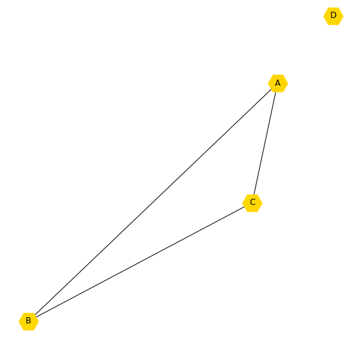

We discussed above changing the colour of the nodes in our graph. There are several ways you can specify colour in Python (matplotlib: node shapes). The RGB format is one of these methods used for specifying a colour. The colour is specified via an array of length 3 containing the relative amounts of Red, Green, and Blue. Red is specified via \([[1, 0, 0]]\), blue via \([[0, 0, 1]]\) and green via \([[0, 1, 0]]\). As special cases, \([[0, 0, 0]]\) will give you black, and \([[1, 1, 1]]\) will give white.

Do it Yourself

Add an edge to the network to connect the isolated node D to e.g. node A.

DIY ANSWER

PYTHON

new_graph.add_edge(3, 0)

nx.draw(new_graph, newLayout,
        labels=newLabels,
        node_color='gold',
        node_shape="H",
        node_size=800);

show()

Instead of altering individual elements of a matrix with zeroes (as we have done above) you can also create a graph directly from a Numpy array. You set up a nested list and convert it to a Numpy array using array.

PYTHON

from numpy import array

matrixFromArray =  array([[0, 1, 0, 0],
                          [0, 1, 0, 1],
                          [1, 0, 1, 1],
                          [1, 0, 1, 0]])

my_graph = nx.from_numpy_matrix(matrixFromArray, create_using=nx.DiGraph())

my_graphLayout = nx.spring_layout(my_graph)

nx.draw(my_graph, my_graphLayout)

show()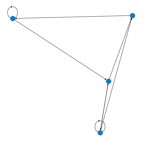

Do it Yourself

Set all the nodes in this graph to turquoise diamonds. By turquoise we mean the RGB colour \([[0, 1, 1]]\)

DIY ANSWER

PYTHON

nx.draw(my_graph, newLayout,
        labels=newLabels,
        node_color=[[0, 1, 1]],
        node_shape="D",
        node_size=800)
show()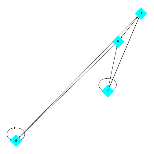

A number of prototypic networks are the fully connected network (each node is connected to all other nodes); the random network (each node is connected to a random subset of other nodes); and the Watts-Strogatz network (a network with a combination of systematically and randomly assigned edges). They are demonstrated in a video tutorial accompanying this Lesson.

Directed graphs

---

So far, we have been working with undirected graphs: all the edges between the nodes were independent of the direction in which they were set up and thus represented as lines without arrowheads. Such networks are also referred to as bidirectional. For some systems, such as biochemical reactions, a directed graph is more suited, and gives us more detail on the relationships represented in the network.

In NetworkX, directed graphs are handled using the class DiGraph. We can make a simple DiGraph by importing a matrix as above, but specifying that it is a directed graph.

PYTHON

directedMatrix =  array([[0, 1, 0, 1],
                         [0, 1, 1, 0],
                         [0, 0, 0, 1],
                         [1, 1, 0, 0]])

directed = nx.from_numpy_matrix(directedMatrix, create_using=nx.DiGraph)

directedLayout = nx.spiral_layout(directed)

directedLabels = {
    0: 'A',
    1: 'B',
    2: 'C',
    3: 'D',
}

nx.draw(directed, directedLayout,
        labels=directedLabels)

show()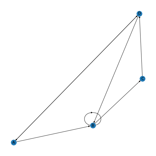

You’ll be able to see in this graph that the edges now have arrow tips indicating the direction of the edge. The edge between node A and node D has an arrow tip on each end, indicating that edge is bidirectional. Node B is also connected to itself.

In NetworkX convention an edge is set up in a network matrix in the direction row \(\rightarrow\) column. Thus, a given row tells us which edges leave the node with that row number. A given column tells us which edges arrive at the node with that column number. Thus the bidirectional edge between node A and node D is given by directedMatrix\(_{3,0}\) and directedMatrix\(_{0,3}\) both being equal to 1.

An entry on the diagonal, directedMatrix\(_{1,1}\), is used for self-connection of node B.

Do it Yourself

Change directedMatrix\(_{3,2}\) to 1. What does this change about the graph?

DIY ANSWER

PYTHON

directedMatrix =  array([[0, 1, 0, 1],
                         [0, 1, 1, 0],
                         [0, 0, 0, 1],
                         [1, 1, 0, 0]])

directedMatrix[3, 2] = 1

directed = nx.from_numpy_matrix(directedMatrix, create_using=nx.DiGraph)

directedLayout = nx.spiral_layout(directed)

directedLabels = {
    0: 'A',
    1: 'B',
    2: 'C',
    3: 'D',
}

nx.draw(directed, directedLayout,
        labels=directedLabels)
show()

Bipartite graphs

---

Bipartite graphs are another graph type supported by NetworkX. These are networks which are made up of two groups of nodes which connect to nodes in the other group, but not with other nodes in the same group. Some ecological, biomedical, and epidemiological networks may be represented by bipartite networks. In NetworkX there is not a specific bipartite class of graphs, but both the undirected and directed methods we have used earlier may be used to represent bipartite graphs. However, it is recommended to add an attribute to the nodes in your two groups to help you differentiate them. The convention in NetworkX is to assign one group of nodes an attribute of 0, and the other an attribute of 1.

PYTHON

from networkx.algorithms import bipartite

myBipartite = nx.Graph()

# Add nodes with the node attribute "bipartite"
myBipartite.add_nodes_from(['h', 'i', 'j', 'k'], bipartite=0)
myBipartite.add_nodes_from(['q', 'r', 's', 't'], bipartite=1)

# Add edges only between nodes of opposite node sets
myBipartite.add_edges_from([('h', 'q'),
                            ('h', 'r'),
                            ('i', 'r'),
                            ('i', 's'),
                            ('j', 's'),
                            ('k', 'q'),
                            ('h', 't')])

Here, we set up a bipartite network with 8 nodes. The 0 group has nodes \('h', 'i', 'j', 'k'\), and the 1 group has nodes \('q', 'r', 's', 't'\). The specified edges link nodes from the two groups with each other, but not to any nodes within their own group. NetworkX has a function to check your nodes are connected.

PYTHON

nx.is_connected(myBipartite)

OUTPUT

True

This will return either true or false. Be cautious though, this only tests for connection, not whether your graph is truly bipartite. You can use the function nx.is_bipartite(myBipartite) from networkx.algorithms to test whether your network is bipartite. It will return TRUE if your NetworkX object is bipartite.

PYTHON

bipartite.is_bipartite(myBipartite)

OUTPUT

True

We can now plot the bipartite graph, using the layout of your choice. if we include the term \(with\_labels = True\) as we draw the graph, the node names we set earlier become the node labels.

PYTHON

myBipartiteLayout = nx.spiral_layout(myBipartite)

nx.draw(myBipartite, myBipartiteLayout,
        node_size=2000,
        with_labels=True)

show()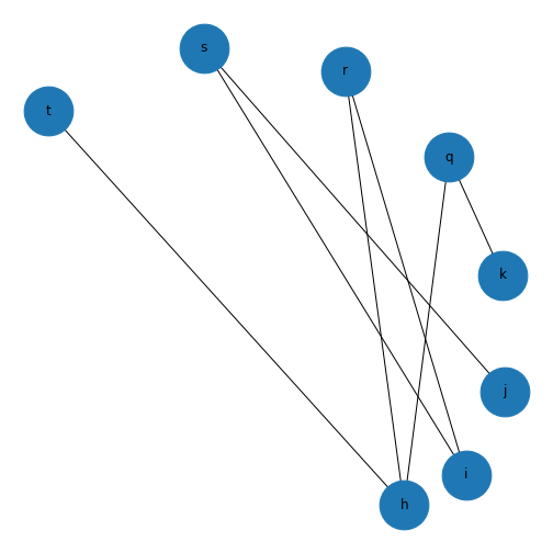

This might not look like a bipartite network! But if you check the edges you set up earlier, this is bipartite as no node has an edge with another node in each group. If we want it to look more like a classic bipartite network, we can use the attributes we set up earlier and the module \(networkx.algorithms\) to make a custom layout and more clearly visualise the bipartite nature of this graph.

PYTHON

groupzero = nx.bipartite.sets(myBipartite)[0]

bipartitePos = nx.bipartite_layout(myBipartite, groupzero)

nx.draw(myBipartite, bipartitePos,
        node_size=2000,
        with_labels = True)

show()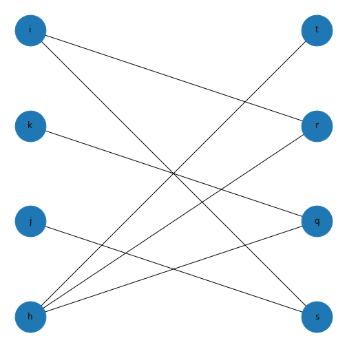

Using the bipartite convention of giving one group of nodes the attribute 0 and the other 1 means that you can use this to change other aspects of your graph, such as colour. Here, we use the attributes of the nodes to assign a colour to each group of nodes. The colour list can then be included in the plot.

PYTHON

color_dictionary = {0: 'gold', 1: 'lavender'}

color_list = list()

for attr in myBipartite.nodes.data('bipartite'):

    color_list.append(color_dictionary[attr[1]])

print(color_list)

OUTPUT

['gold', 'gold', 'gold', 'gold', 'lavender', 'lavender', 'lavender', 'lavender']

PYTHON

nx.draw(myBipartite, bipartitePos,
        node_size=2000,
        font_size=20,
        with_labels=True,
        node_color=color_list)

show()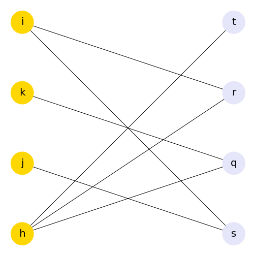

A readable introduction to bipartite networks and their application to gene-disease networks can be found in section 2.7 of the online textbook Network Science by A.L. Barabási.

Exercises

---

Assignment: the Toxin-Antitoxin Network

Use code to create the (undirected) toxin-antitoxin PPI network given at the start of this example. Experiment with the different layout algorithms, the node colour and shape, and the edge color.

Hint:

• Using pen and paper, draw a diagram of the PPI network.
• Decide on the ordering of the nodes. I chose to start with the centre node, and then number them in an anticlockwise direction. (Hint: There are 11 nodes in total.)
• Label your pen and paper diagram with the node numbers.
• Work out all the edges in the graph. Note the numbers of the node at the start of the edge and the node at the end of the edge. (Hint: There are 20 edges in total.)
• Define a \(11 \times 11\) matrix in Python using the Numpy zeros function.
• For each edge, set the corresponding entry in the matrix to 1 (start node number corresponds to row number and end node number corresponds to column number in the adjacency matrix).
• Define a cell array containing your node names and create a NetworkX object.
• Experiment with the layout, colours, node shapes etc.

Remember to use the Python documentation, e.g. using help() if you have problems (or alternatively use a search engine such as Google).

To save the graph as an image file, use savefig as we did earlier.

Please check these solutions only after submitting the assignments.

PYTHON

import networkx as nx

from numpy import zeros

ppi = zeros((11,11))

ppiLabels = {
    0: 'mazG',
    1: 'mazE',
    2: 'mazF',
    3: 'relA',
    4: 'era',
    5: 'rpo2',
    6: 'dcd',
    7: 'pyrG',
    8: 'adk',
    9: 'cpdA',
    10: 'ygdH',
}

ppi[0, 1] = 1
ppi[2, 1] = 1
ppi[0, 2] = 1
ppi[2, 3] = 1
ppi[0, 3] = 1
ppi[1, 3] = 1
ppi[4, 3] = 1
ppi[5, 3] = 1
ppi[4, 0] = 1
ppi[5, 0] = 1
ppi[5, 6] = 1
ppi[5, 7] = 1
ppi[0, 7] = 1
ppi[8, 7] = 1
ppi[8, 0] = 1
ppi[8, 9] = 1
ppi[8, 10] = 1
ppi[0, 9] = 1
ppi[9, 10] = 1
ppi[0, 10] = 1

ppiGraph = nx.from_numpy_matrix(ppi)

ppiLayout = nx.spring_layout(ppiGraph)

nx.draw(ppiGraph, ppiLayout,
              labels=ppiLabels,
              node_size=1800,
              node_color='lightseagreen',
              node_shape="8")

show()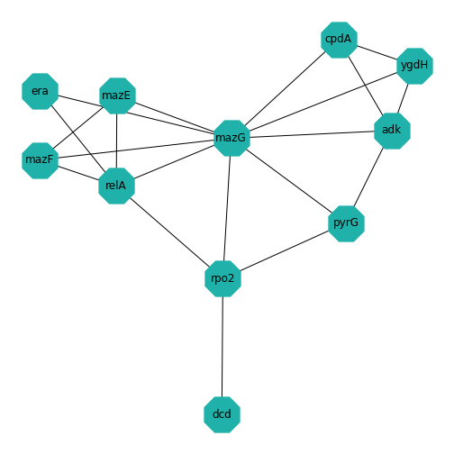

Key Points

• A Python package NetworkX is used for studying undirected and directed graphs.
• A function savefig is used to save a graph to a file.
• network matrix or adjacency matrix is a generic way to create graphs as two dimensional array.
• In NetworkX, directed graphs are handled using the class DiGraph.
• Bipartite graphs are made up of two groups of nodes which connect to nodes in the other group, but not with other nodes in the same group.